Excel dashboards are powerful when done right. They’re also time-consuming to build, fragile when data changes, and hard to share without handing over the whole file. This tutorial shows you how to build a proper Excel dashboard from scratch — then shows you what the same result looks like when you let AI handle it.

Before You Build: Data Prep

The most common reason Excel dashboards break is bad data structure. Your raw data needs:

• One row per record — no summary rows mixed into your data table
• Consistent date formats — Excel treats March 2026, 03/2026, and 2026-03 as three different values
• No merged cells — they break pivot tables
• Headers in row 1 — no blank rows at the top

If your data is messy, clean it first. Use Power Query (Data → Get & Transform Data) to normalize formats, remove blanks, and combine tables. Time spent here saves hours of debugging later.

Step 1: Convert Data to a Table

Select your data range and press Ctrl+T (Cmd+T on Mac). This converts it to a named Excel Table, which automatically expands when you add rows. Name it something useful — SalesData, MonthlyRevenue — rather than the default Table1.

Structured tables are the foundation of everything else. Pivot tables, charts, and formulas all behave better when they reference a named table instead of a static range.

Step 2: Build Pivot Tables for Each Metric

Pivot tables are how you summarize large datasets without writing complex formulas. For an Excel dashboard, you typically need one pivot table per visualization.

Insert → PivotTable → From Table/Range

Choose “New Worksheet” and give the sheet a name like PT_Revenue. Build the pivot by dragging fields:

• Rows: Date (grouped by month)
• Values: Revenue (Sum)

Repeat this process for each metric you need: sales by region, units by product, conversions by channel. Keep each pivot table on its own sheet — don’t stack them on the same tab.

Step 3: Build the Chart Layer

With a pivot table selected, go to Insert → PivotChart. Excel builds a chart that stays connected to the pivot. For dashboards:

• Line chart → trend over time
• Clustered bar chart → comparison across categories
• Donut or pie chart → use only for 2-3 segments max

Move each chart to your Dashboard sheet. Right-click the chart frame → Move Chart → Object in → select your Dashboard tab.

Step 4: Add Slicers for Interactivity

Slicers are the easiest way to add filters to an Excel dashboard without touching VBA.

Click a pivot table → Insert → Slicer. Select the fields you want to filter by: date range, region, product category, rep name.

Position slicers at the top or side of your dashboard. Then right-click each slicer → Report Connections → connect it to all pivot tables so one click filters everything simultaneously.

This is what turns a static chart collection into an actual dashboard.

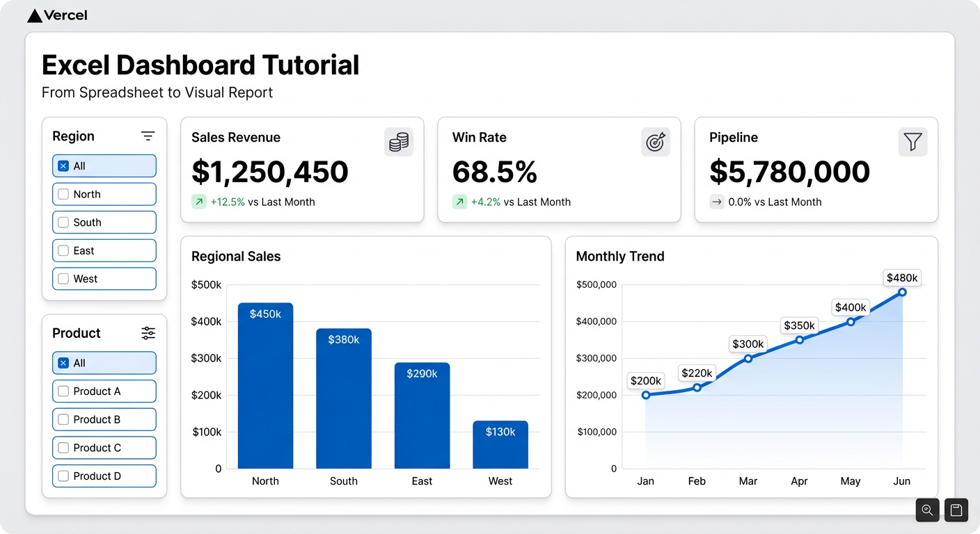
Step 5: Design the Dashboard Tab

Create a dedicated Dashboard tab. This is what people see — keep the data tabs hidden.

Design principles that actually matter:

• White background — remove gridlines (View → Gridlines, uncheck)
• Align everything to a grid — unaligned charts look amateur
• Limit to one accent colour — use it for key metrics only
• Put the most important number at the top-left — that’s where eyes go first

Add KPI boxes using simple cells with large bold fonts. Reference your pivot table values directly with formulas: =PT_Revenue!B5. Format the cells with borders and background fill to make them look like metric cards.

Step 6: Lock and Share

Protect the Dashboard sheet: Review → Protect Sheet. Let viewers select cells but not edit them.

Hide the Pivot Table sheets and Data sheet: right-click the tab → Hide.

For sharing, export as PDF for a snapshot, or share the file with specific people via OneDrive for a live version. The problem: sharing the file means sharing all your data, protected or not. Anyone with edit access can unprotect and dig through everything.

Where Excel Dashboards Fall Short

Excel dashboards work. For internal reporting where everyone has Excel and the data doesn’t change often, they’re fine.

But they break down when:

• Data updates frequently — someone has to manually paste in new numbers
• You need to share with non-Excel users — the recipient has to have the right Excel version
• Charts need to look good on any screen — Excel charts don’t scale cleanly for presentations
• Multiple people need the same dashboard — file sharing gets messy fast

Build the Same Dashboard in Two Minutes

If your data is already in Excel — or in Excel Online — Infograph connects directly and builds from a prompt.

Connect your Microsoft account, select your Excel file, type what you want to see. The dashboard builds instantly and stays live: when your spreadsheet updates, the dashboard updates. Share it with a link, not a file.

No pivot tables. No slicer configuration. No protected sheets. The process that takes two hours in Excel takes two minutes with AI.

Try this with your own data at app.infograph.ai.